
1편가기 (현재 블록체인 분야에 집중하고 있어서 2편 번역 할 시간이 없네요.. 죄송합니다 ㅜㅜ)
Part II: Advanced concepts
We now have a very good intuition of what convolution is, and what is going on in convolutional nets, and why convolutional nets are so powerful. But we can dig deeper to understand what is really going on within a convolution operation. In doing so, we will see that the original interpretation of computing a convolution is rather cumbersome and we can develop more sophisticated interpretations which will help us to think about convolutions much more broadly so that we can apply them on many different data. To achieve this deeper understanding the first step is to understand the convolution theorem.
The convolution theorem
To develop the concept of convolution further, we make use of the convolution theorem, which relates convolution in the time/space domain — where convolution features an unwieldy integral or sum — to a mere element wise multiplication in the frequency/Fourier domain. This theorem is very powerful and is widely applied in many sciences. The convolution theorem is also one of the reasons why the fast Fourier transform (FFT) algorithm is thought by some to be one of the most important algorithms of the 20th century.
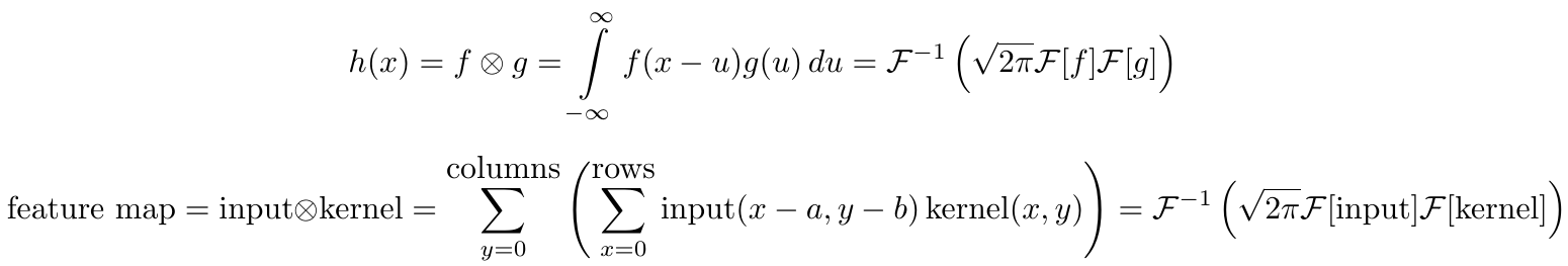
The first equation is the one dimensional continuous convolution theorem of two general continuous functions; the second equation is the 2D discrete convolution theorem for discrete image data. Here 


To get a better understanding what happens in the convolution theorem we will now look at the interpretation of Fourier transforms with respect to digital image processing.
Fast Fourier transforms
The fast Fourier transform is an algorithm that transforms data from the space/time domain into the frequency or Fourier domain. The Fourier transform describes the original function in a sum of wave-like cosine and sine terms. It is important to note, that the Fourier transform is generally complex valued, which means that a real value is transformed into a complex value with a real and imaginary part. Usually the imaginary part is only important for certain operations and to transform the frequencies back into the space/time domain and will be largely ignored in this blog post. Below you can see a visualization how a signal (a function of information often with a time parameter, often periodic) is transformed by a Fourier transform.
You may be unaware of this, but it might well be that you see Fourier transformed values on a daily basis: If the red signal is a song then the blue values might be the equalizer bars displayed by your mp3 player.
The Fourier domain for images
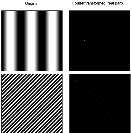
How can we imagine frequencies for images? Imagine a piece of paper with one of the two patterns from above on it. Now imagine a wave traveling from one edge of the paper to the other where the wave pierces through the paper at each stripe of a certain color and hovers over the other. Such waves pierce the black and white parts in specific intervals, for example, every two pixels — this represents the frequency. In the Fourier transform lower frequencies are closer to the center and higher frequencies are at the edges (the maximum frequency for an image is at the very edge). The location of Fourier transform values with high intensity (white in the images) are ordered according to the direction of the greatest change in intensity in the original image. This is very apparent from the next image and its log Fourier transforms (applying the log to the real values decreases the differences in pixel intensity in the image — we see information more easily this way).
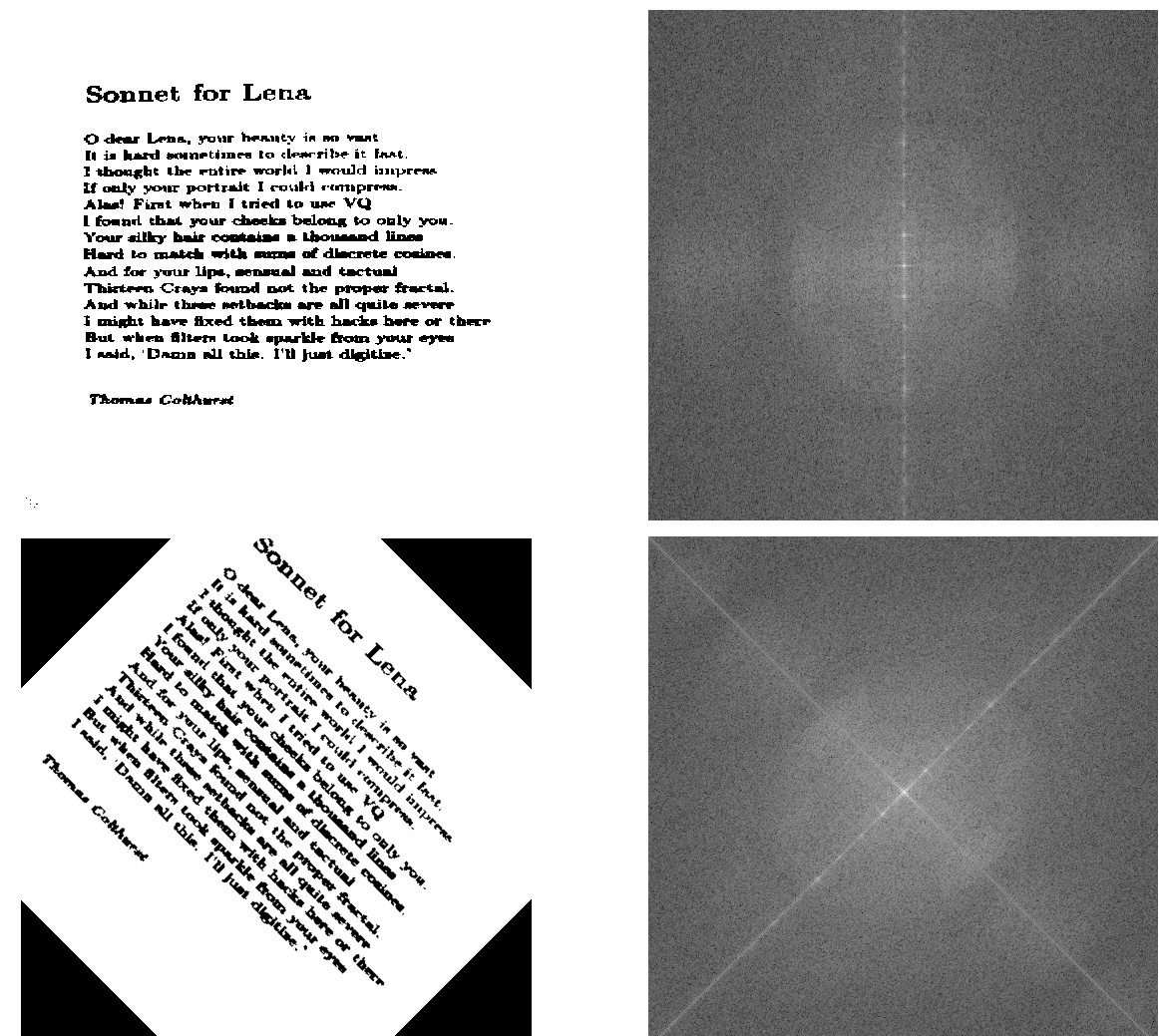
We immediately see that a Fourier transform contains a lot of information about the orientation of an object in an image. If an object is turned by, say, 37% degrees, it is difficult to tell that from the original pixel information, but very clear from the Fourier transformed values.
This is an important insight: Due to the convolution theorem, we can imagine that convolutional nets operate on images in the Fourier domain and from the images above we now know that images in that domain contain a lot of information about orientation. Thus convolutional nets should be better than traditional algorithms when it comes to rotated images and this is indeed the case (although convolutional nets are still very bad at this when we compare them to human vision).
Frequency filtering and convolution
The reason why the convolution operation is often described as a filtering operation, and why convolution kernels are often named filters will be apparent from the next example, which is very close to convolution.
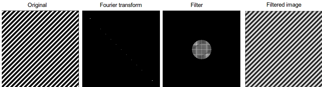
If we transform the original image with a Fourier transform and then multiply it by a circle padded by zeros (zeros=black) in the Fourier domain, we filter out all high frequency values (they will be set to zero, due to the zero padded values). Note that the filtered image still has the same striped pattern, but its quality is much worse now — this is how jpeg compression works (although a different but similar transform is used), we transform the image, keep only certain frequencies and transform back to the spatial image domain; the compression ratio would be the size of the black area to the size of the circle in this example.
If we now imagine that the circle is a convolution kernel, then we have fully fledged convolution — just as in convolutional nets. There are still many tricks to speed up and stabilize the computation of convolutions with Fourier transforms, but this is the basic principle how it is done.
Now that we have established the meaning of the convolution theorem and Fourier transforms, we can now apply this understanding to different fields in science and enhance our interpretation of convolution in deep learning.
Insights from fluid mechanics
Fluid mechanics concerns itself with the creation of differential equation models for flows of fluids like air and water (air flows around an airplane; water flows around suspended parts of a bridge). Fourier transforms not only simplify convolution, but also differentiation, and this is why Fourier transforms are widely used in the field of fluid mechanics, or any field with differential equations for that matter. Sometimes the only way to find an analytic solution to a fluid flow problem is to simplify a partial differential equation with a Fourier transform. In this process we can sometimes rewrite the solution of such a partial differential equation in terms of a convolution of two functions which then allows for very easy interpretation of the solution. This is the case for the diffusion equation in one dimension, and for some two dimensional diffusion processes for functions in cylindrical or spherical polar coordinates.
Diffusion
You can mix two fluids (milk and coffee) by moving the fluid with an outside force (mixing with a spoon) — this is called convection and is usually very fast. But you could also wait and the two fluids would mix themselves on their own (if it is chemically possible) — this is called diffusion and is usually a very slow when compared to convection.
Imagine an aquarium that is split into two by a thin, removable barrier where one side of the aquarium is filled with salt water, and the other side with fresh water. If you now remove the thin barrier carefully, the two fluids will mix together until the whole aquarium has the same concentration of salt everywhere. This process is more “violent” the greater the difference in saltiness between the fresh water and salt water.
Now imagine you have a square aquarium with 256×256 thin barriers that separate 256×256 cubes each with different salt concentration. If you remove the barrier now, there will be little mixing between two cubes with little difference in salt concentration, but rapid mixing between two cubes with very different salt concentrations. Now imagine that the 256×256 grid is an image, the cubes are pixels, and the salt concentration is the intensity of each pixel. Instead of diffusion of salt concentrations we now have diffusion of pixel information.
It turns out, this is exactly one part of the convolution for the diffusion equation solution: One part is simply the initial concentrations of a certain fluid in a certain area — or in image terms — the initial image with its initial pixel intensities. To complete the interpretation of convolution as a diffusion process we need to interpret the second part of the solution to the diffusion equation: The propagator.
Interpreting the propagator
The propagator is a probability density function, which denotes into which direction fluid particles diffuse over time. The problem here is that we do not have a probability function in deep learning, but a convolution kernel — how can we unify these concepts?
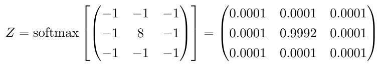
We can apply a normalization that turns the convolution kernel into a probability density function. This is just like computing the softmax for output values in a classification tasks. Here the softmax normalization for the edge detector kernel from the first example above.
Now we have a full interpretation of convolution on images in terms of diffusion. We can imagine the operation of convolution as a two part diffusion process: Firstly, there is strong diffusion where pixel intensities change (from black to white, or from yellow to blue, etc.) and secondly, the diffusion process in an area is regulated by the probability distribution of the convolution kernel. That means that each pixel in the kernel area, diffuses into another position within the kernel according to the kernel probability density.
For the edge detector above almost all information in the surrounding area will concentrate in a single space (this is unnatural for diffusion in fluids, but this interpretation is mathematically correct). For example all pixels that are under the 0.0001 values, will very likely flow into the center pixel and accumulate there. The final concentration will be largest where the largest differences between neighboring pixels are, because here the diffusion process is most marked. In turn, the greatest differences in neighboring pixels is there, where the edges between different objects are, so this explains why the kernel above is an edge detector.
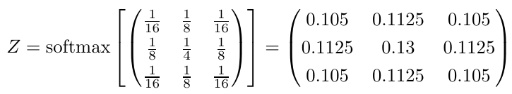
So there we have it: Convolution as diffusion of information. We can apply this interpretation directly on other kernels. Sometimes we have to apply a softmax normalization for interpretation, but generally the numbers in itself say a lot about what will happen. Take the following kernel for example. Can you now interpret what that kernel is doing? Click here to find the solution (there is a link back to this position).
Wait, there is something fishy here
How come that we have deterministic behavior if we have a convolution kernel with probabilities? We have to interpret that single particles diffuse according to the probability distribution of the kernel, according to the propagator, don’t we?
Yes, this is indeed true. However, if you take a tiny piece of fluid, say a tiny drop of water, you still have millions of water molecules in that tiny drop of water, and while a single molecule behaves stochastically according to the probability distribution of the propagator, a whole bunch of molecules have quasi deterministic behavior —this is an important interpretation from statistical mechanics and thus also for diffusion in fluid mechanics. We can interpret the probabilities of the propagator as the average distribution of information or pixel intensities; Thus our interpretation is correct from a viewpoint of fluid mechanics. However, there is also a valid stochastic interpretation for convolution.
Insights from quantum mechanics
The propagator is an important concept in quantum mechanics. In quantum mechanics a particle can be in a superposition where it has two or more properties which usually exclude themselves in our empirical world: For example, in quantum mechanics a particle can be at two places at the same time — that is a single object in two places.
However, when you measure the state of the particle — for example where the particle is right now — it will be either at one place or the other. In other terms, you destroy the superposition state by observation of the particle. The propagator then describes the probability distribution where you can expect the particle to be. So after measurement a particle might be — according to the probability distribution of the propagator — with 30% probability in place A and 70% probability in place B.
If we have entangled particles (spooky action at a distance), a few particles can hold hundreds or even millions of different states at the same time — this is the power promised by quantum computers.
So if we use this interpretation for deep learning, we can think that the pixels in an image are in a superposition state, so that in each image patch, each pixel is in 9 positions at the same time (if our kernel is 3×3). Once we apply the convolution we make a measurement and the superposition of each pixel collapses into a single position as described by the probability distribution of the convolution kernel, or in other words: For each pixel, we choose one pixel of the 9 pixels at random (with the probability of the kernel) and the resulting pixel is the average of all these pixels. For this interpretation to be true, this needs to be a true stochastic process, which means, the same image and the same kernel will generally yield different results. This interpretation does not relate one to one to convolution but it might give you ideas how to the apply convolution in stochastic ways or how to develop quantum algorithms for convolutional nets. A quantum algorithm would be able to calculate all possible combinations described by the kernel with onecomputation and in linear time/qubits with respect to the size of image and kernel.
Insights from probability theory
Convolution is closely related to cross-correlation. Cross-correlation is an operation which takes a small piece of information (a few seconds of a song) to filter a large piece of information (the whole song) for similarity (similar techniques are used on youtube to automatically tag videos for copyrights infringements).
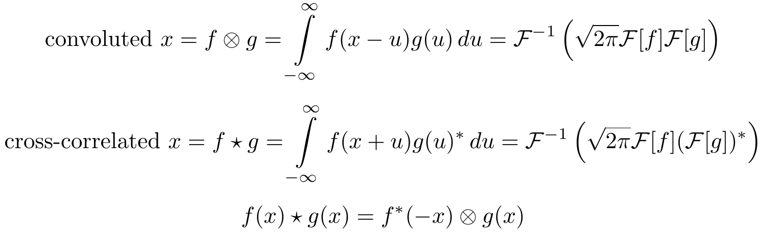
While cross correlation seems unwieldy, there is a trick with which we can easily relate it to convolution in deep learning: For images we can simply turn the search image upside down to perform cross-correlation through convolution. When we perform convolution of an image of a person with an upside image of a face, then the result will be an image with one or multiple bright pixels at the location where the face was matched with the person.
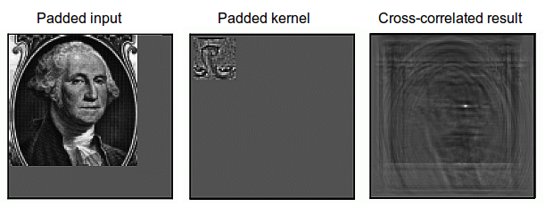
This example also illustrates padding with zeros to stabilize the Fourier transform and this is required in many version of Fourier transforms. There are versions which require different padding schemes: Some implementation warp the kernel around itself and require only padding for the kernel, and yet other implementations perform divide-and-conquer steps and require no padding at all. I will not expand on this; the literature on Fourier transforms is vast and there are many tricks to be learned to make it run better — especially for images.
At lower levels, convolutional nets will not perform cross correlation, because we know that they perform edge detection in the very first convolutional layers. But in later layers, where more abstract features are generated, it is possible that a convolutional net learns to perform cross-correlation by convolution. It is imaginable that the bright pixels from the cross-correlation will be redirected to units which detect faces (the Google brain project has some units in its architecture which are dedicated to faces, cats etc.; maybe cross correlation plays a role here?).
Insights from statistics
What is the difference between statistical models and machine learning models? Statistical models often concentrate on very few variables which can be easily interpreted. Statistical models are built to answer questions: Is drug A better than drug B?
Machine learning models are about predictive performance: Drug A increases successful outcomes by 17.83% with respect to drug B for people with age X, but 22.34% for people with age Y.
Machine learning models are often much more powerful for prediction than statistical models, but they are not reliable. Statistical models are important to reach accurate and reliable conclusions: Even when drug A is 17.83% better than drug B, we do not know if this might be due to chance or not; we need statistical models to determine this.
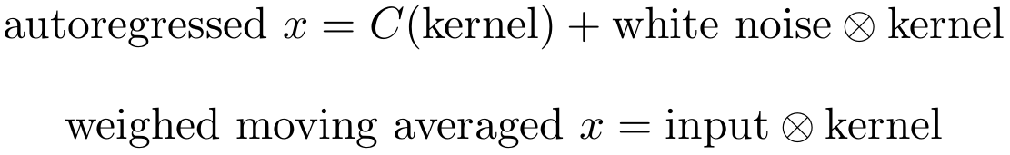
Two important statistical models for time series data are the weighted moving average and the autoregressive models which can be combined into the ARIMA model (autoregressive integrated moving average model). ARIMA models are rather weak when compared to models like long short-term recurrent neural networks, but ARIMA models are extremely robust when you have low dimensional data (1-5 dimensions). Although their interpretation is often effortful, ARIMA models are not a blackbox like deep learning algorithms and this is a great advantage if you need very reliable models.
It turns out that we can rewrite these models as convolutions and thus we can show that convolutions in deep learning can be interpreted as functions which produce local ARIMA features which are then passed to the next layer. This idea however, does not overlap fully, and so we must be cautious and see when we really can apply this idea.
Here }")
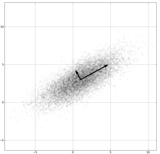
When we pre-process data we make it often very similar to white noise: We often center it around zero and set the variance/standard deviation to one. Creating uncorrelated variables is less often used because it is computationally intensive, however, conceptually it is straight forward: We reorient the axes along the eigenvectors of the data.
Now, if we take
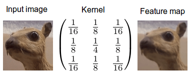
The interpretation of the weighted moving average is simple: It is just standard convolution on some data (input) with a certain weight (kernel). This interpretation becomes clearer when we look at the Gaussian smoothing kernel at the end of the page. The Gaussian smoothing kernel can be interpreted as a weighted average of the pixels in each pixel’s neighborhood, or in other words, the pixels are averaged in their neighborhood (pixels “blend in”, edges are smoothed).
While a single kernel cannot create both, autoregressive and weighted moving average features, we usually have multiple kernels and in combination all these kernels might contain some features which are like a weighted moving average model and some which are like an autoregressive model.
Conclusion
In this blog post we have seen what convolution is all about and why it is so powerful in deep learning. The interpretation of image patches is easy to understand and easy to compute but it has many conceptual limitations. We developed convolutions by Fourier transforms and saw that Fourier transforms contain a lot of information about orientation of an image. With the powerful convolution theorem we then developed an interpretation of convolution as the diffusion of information across pixels. We then extended the concept of the propagator in the view of quantum mechanics to receive a stochastic interpretation of the usually deterministic process. We showed that cross-correlation is very similar to convolution and that the performance of convolutional nets may depend on the correlation between feature maps which is induced through convolution. Finally, we finished with relating convolution to autoregressive and moving average models.
Personally, I found it very interesting to work on this blog post. I felt for long time that my undergraduate studies in mathematics and statistics were wasted somehow, because they were so unpractical (even though I study applied math). But later — like an emergent property — all these thoughts linked together and practically useful understanding emerged. I think this is a great example why one should be patient and carefully study all university courses — even if they seem useless at first.

